Development of a physical district energy network model
Background and motivation
A District Energy (DE) grid is a centralized energy management system consisting of a network of buried pipes, which permits the sharing of energy sources and loads between all buildings connected. High energy efficiencies are achieved in DE grids as loads (i.e. heating, cooling, or electricity, or any combination thereof) are aggregated, allowing greater run-time for base-load energy plants); various heat recovery and energy storage technologies can also be integrated into DE grids for increasing overall energy efficiency.
Hourly simulation tools are currently in widespread use by industry for predicting energy flows, sizing components, and determining fuel requirements in proposed DE systems. Although considered the norm in this sector, low resolution DE simulation models (i.e. models with time steps of 1 hour or greater) cannot properly account for the effects of varying flow and thermal inertia in the system. As a consequence, averaging effects are incurred resulting in misleading economic and environmental outcomes. To address this problem, a high resolution numerical tool (i.e. a model with time steps ranging from 1 – 60 seconds) has been developed which can simulate dynamic conditions in a DE grids. The tool can determine system heat storage capability as a function of time and calculate heat dissipation and pressure at different points in the grid.
Model description
The DE network model simulates the performance of a dual pipe, supply-return DE system. A variable transport delay is used in the model to assess time-varying fluid flow response in the network. Water is used as the fluid medium in the model. With an allowable fluid temperature range of (0°C – 100°C), the model is appropriate for simulating both ambient temperature (5°C – 25°C) DE systems and medium temperature (50°C – 90°C) DE systems. Ambient temperature DE systems deliver energy to building loads via heat pumps, whereas medium temperature DE systems use heat exchangers. Model inputs are thermal source capacities, building heating loads, outside temperature, pipe characteristics (i.e. pipe assembly material properties, dimensions, and burial depth), and soil characteristics. Thermal sources available in the model are Combined Heat and Power (CHP) plants, heat recovery plants, and boiler plants. Model outputs are fluid temperature, pressure, and mass flow rate (at user-defined nodes in the network), piping network heat losses, pumping energy requirements, fuel requirements, and CO2 emissions. All pumps in the DE network are variable speed types and are either pressure controlled or temperature controlled. A pressure controlled Variable Speed Pump (VSP) varies its flow to maintain a set differential pressure in a valve chamber located at the end of the piping circuit. Alternatively, a temperature controlled VSP varies its flow to maintain a set differential temperature on the DE side of the building heat exchanger.
Model validation
The CRD ‘Saanich’ DE system, located on Vancouver Island, BC, is modeled using the DE network model for validation purposes; it is a low temperature, effluent heat recovery system that uses water as the flow medium. A schematic of the Saanich DE system is shown in Figure 1. Heat (depicted as QS in Figure 1) is transferred to the DE system from the effluent via a heat exchanger bank located in the heat recovery plant. The DE system services a single load (i.e. a pool), shown as QL in Figure 1, for which energy is supplied via a heat pump located in the pool miniplant. Figure 1 also depicts a tee junction, which separates the heat recovery circuit from the miniplant circuit, and a valve chamber, which controls the Variable Speed Pump (VSP) in the heat recovery plant. Contrary to the heat recovery circuit, the miniplant circuit uses a Constant Speed Pump (CSP).
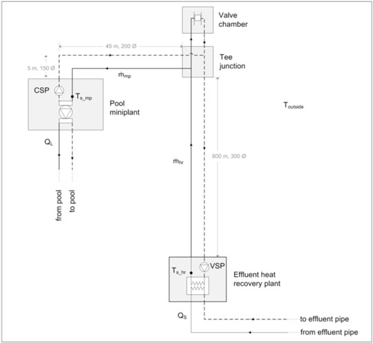
Figure 1: Saanich district energy system schematic
The piping network in the Saanich DE system consists of un-insulated HDPE pipe, buried at an approximate depth of 1.2 m. The total distance between the effluent heat recovery plant and the miniplant is approximately 850 m; the nominal pipe diameter is reduced over this distance from 300 mm to 200 mm to 150 mm, as shown in Figure 1.
Validation results
The Saanich DE network model is a minute time step model; it is used to validate the DE pipe heat transfer model, head loss model, and variable transport delay. Model inputs are outside temperature, miniplant heat load, heat recovery plant supply temperature, heat recovery circuit mass flow rate, and miniplant circuit mass flow rate; shown as Toutside, QL, Ts_hr, ṁhr, and ṁmp, respectively, in Figure 1. Validation parameters are the miniplant supply temperature, Ts_mp (depicted in Figure 1), and hTotal, the total head loss in the heat recovery circuit. All system data is obtained from the Saanich online SCADA system, which is used for sampling and monitoring data from remote sensors located throughout the Saanich DE system. Measured versus calculated data for Ts_mp are shown in Figure 2 for January 2nd, 2012. Figure 2 shows that the variable transport delay used in the Saanich DE network model fits well with the measured data; the time delay shown between the two datasets is less than approximately 2 minutes on average (possibly due to flow sensor error, specified as ± 1 % by the manufacturer, and/or a linear interpolation error); for comparison, if no variable transport delay were used in the model, the time delay between datasets would be approximately 90 minutes, on average. The calculated temperature in Figure 2 is slightly greater than the measured temperature by approximately 0.2°C on average; this overcompensation may be due to a number of factors such as the error in the temperature sensors (approximately ± 0.2°C from manufacturer specifications), and the error in estimating thermal conductivity for soil and pipe materials in the model.
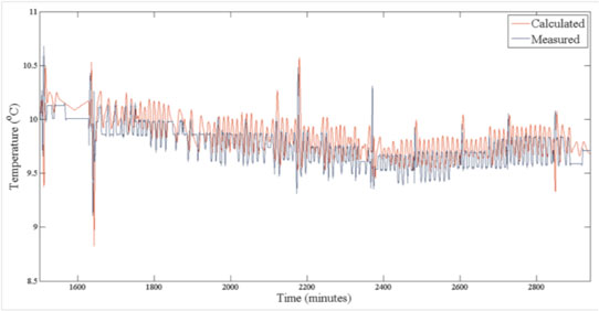
The Probability Density Function (PDF) of the percent difference dataset reveals a standard deviation and mean of 3.8 %, and 1.3 %, respectively.
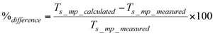
Measured versus calculated data for hTotal are shown in Figure 3 for January 2nd, 2012. Figure 3 shows the magnitude of the calculated dataset as being greater than that of the measured dataset by approximately 0.2 meters on average; the figure also shows the calculated dataset to be periodically increasing and decreasing over a wider head loss range and spiking at various time steps, in contrast to the measured dataset. The difference between datasets in Figure 3 may be due to the following factors: 1) the inability of the DE pipe model to account for the expansion and contraction of the flexible HDPE pipe; 2) the error in the pressure sensors (approximately ± 0.25 % from manufacturer specifications); 3) the error in estimating inner pipe roughness and minor losses in bends and fittings in the model; and 4) the absence of a PID controller model for controlling pump flow in the DE network model. The pressure spikes shown in the calculated dataset of Figure 3 can be due to the flow being adjusted only after every minute time step, as opposed to gradually like what would occur with a PID controller model.
Figure 3: Measured versus calculated data for total head loss in the heat recovery circuit, hTotal, for January 2nd, 2012
A PDF of the % difference “head loss” dataset gives a standard deviation and mean of 6.9 % and 7 %, respectively.
As the calculated validation parameters are within an acceptable range of the measured validation parameters, the model can be used for simulating other DE systems.