Energy Market Modeling using PLEXOS
PLEXOS is object-oriented simulation software used for power market modelling. Thanks to its cutting-edge mathematical programming and stochastic optimization techniques, it can effectively deal with very complex problems and uncertainties (such future load, natural inflow and fuel price). To this end, PLEXOS breaks down a complex problem (e.g. power market modelling over 30 years with one hour resolution) into many sub-problems and solves them in a cascaded manner as shown in Figure 1.
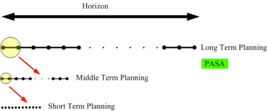
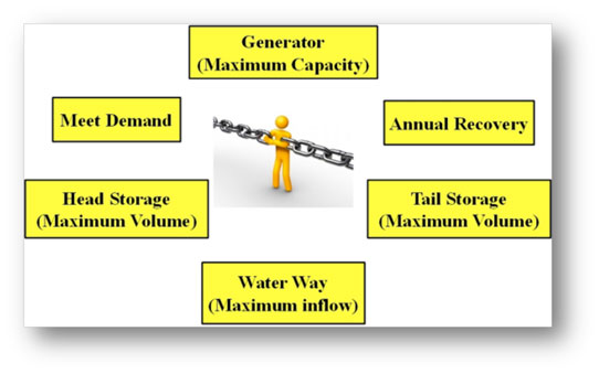
The main purpose for long term planning is capacity expansion on an annual (or user defined) basis. After LT planning and before MT scheduling, Project Assessment System Adequacy (PASA) can be executed which focuses on schedule maintenance events (planned and random outages). Middle term planning is mainly in charge of managing hydro storages, fuel supply and emission constraints on a monthly (or user defined) basis. Finally, ST scheduling deals with dispatch problem and clears the market for every single interval (e.g. every 5 minutes).
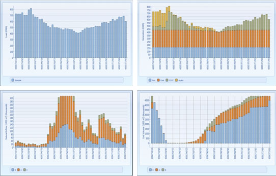
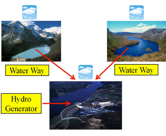
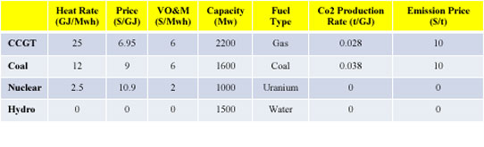
Example: To illustrate the above approach, the energy market for a simple cascaded hydro network along with three thermal generators will be modeled using PLEXOS for a year with one hour resolution. The hydro network consists of a hydro generator and two small storages connected to a large storage through two waterways (Figure 2). The historical natural inflow is available for the last year and the year before. Also, the load forecast is given for the future year. The characteristics of all generators used in this simulation are summarized in Table 1.
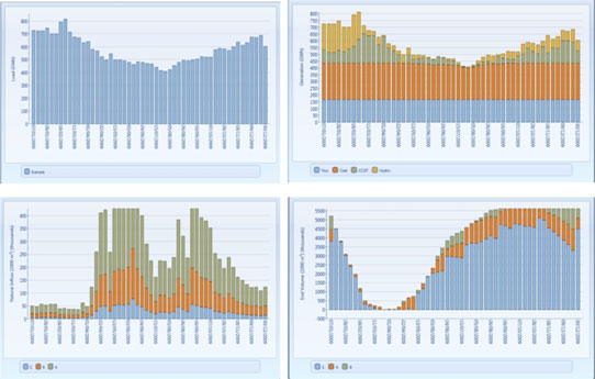
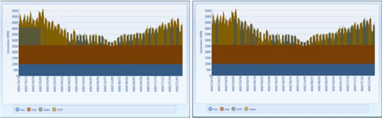
Given limited amount of water, the problem is to find the “best” release policy which minimizes the production cost in the next year (with an hour resolution). This problem can be mathematically modelled as a linear optimization problem with respect to a number of constraints as shown in Figure 3. To significantly reduce the computation load, we can consider a cascaded approach featuring MT and ST planning. The MT (weekly resolution) and ST (hourly resolution) results are shown in Figure 4, 5 and 6 for two different natural inflow scenarios.